An optical resonant cavity is a cavity in which light waves reflect back and forth, thereby providing optical energy feedback. It is a necessary component of a laser, usually composed of two plane or concave spherical mirrors perpendicular to the axis of the active medium.

Figure 1: Properly placing two mirrors (spherical or plane) at both ends of the active medium forms the simplest optical resonator.
The modes of an optical resonator, also called the electromagnetic field distribution in the cavity, can replicate themselves after one complete round trip. Specifically, this means that the amplitude distribution of the electromagnetic field (including the phase of the light) must remain consistent after one round trip, except for possible optical power loss.
These modes exist in geometrically stable resonators, while in unstable resonators their mode characteristics are more complex. In applications such as laser resonators, Fabry-Perot interferometers, and mode cleaners (Figure 2), these modes play a crucial role.

Figure 2: Mode cleaner, composed of two lenses and a pinhole.
In the most basic case, a resonator composed only of parabolic mirrors and a uniform medium has modes that follow Hermite-Gaussian modes. Among them, the most basic mode is the Gaussian mode, whose field distribution is described by a Gaussian function (that is, a Gaussian beam). The changes in beam radius and the radius of curvature of the wavefront depend on the specific design of the resonator.

Figure 3: Shows a simple resonator and the electric field distribution of its Gaussian mode. The wavefront must be planar on the flat left mirror, and the beam radius on the left mirror must match the curvature of the right mirror.
For example, Figures 3 and 4 above show the Gaussian modes of two simple resonators with different configurations composed of a plane mirror, a laser crystal, and a curved end mirror. With a larger end-mirror curvature (as in Figure 4), the mode radius on the left mirror decreases. It can be seen that the beam with a flat wavefront starting from the left side (suitable for a plane mirror) expands as it propagates to the right to match the shape of the other mirror, achieving self-replication of the field configuration including the wavefront shape. In addition, the round-trip phase difference should be an integer multiple of 2π.

Figure 4: Same as Figure 3, but with a larger curvature of the right mirror.
If the right end mirror is bent in the opposite direction (that is, convex), no Gaussian mode exists, and we are facing an unstable resonator. Although this resonator also has modes, their shapes are more complex. Most lasers operate in a stable state with Gaussian modes present in the resonator.
For the above simple resonator, the mode parameters can be calculated through relatively simple equations. However, for more complex resonator configurations, such as those involving multiple curved mirrors and other optical elements (for example, laser crystals with thermal lensing effects), numerical software is usually required to calculate the mode properties.
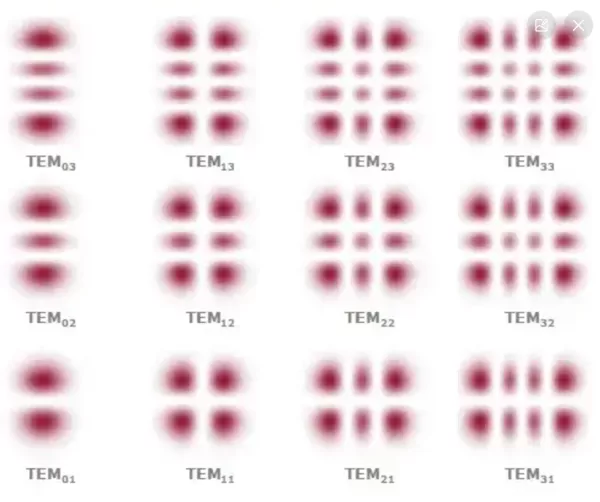
Besides the Gaussian mode, stable resonators also have higher-order modes with more complex intensity distributions. At the beam waist, the electric field distribution can be expressed as the product of two Gaussian functions with orders n and m (non-negative integers, corresponding to the x and y directions respectively). (We still assume a simple resonator containing only parabolic mirrors and an optically uniform medium.) These modes are also called TEMnm modes. The intensity distribution of this mode (as shown in Figure 3) has n nodes in the horizontal direction and m nodes in the vertical direction (as shown in Figure 5).
If the Gaussian beam radius of the fundamental mode is known, the mode distribution of all higher-order modes can be easily calculated.

Figure 5: Intensity distribution of TEMnm modes.
For optical resonance, the amplitude distribution must not only maintain its shape after one round trip, but also undergo a phase change of an integer multiple of 2π. This applies only to specific optical frequencies. Therefore, these modes are characterized by three indices: the transverse mode indices n and m, and the axial mode number q (the round-trip phase change divided by 2π).
In some important cases, we use a notation like TEM_{nmq} to include the axial mode number. When n equals 0 and m equals 0, these modes are called axial modes (or fundamental modes, Gaussian modes), while all other modes are called higher-order modes or higher-order transverse modes.
Please note that, due to the Gouy phase shift, the optical frequency depends not only on the axial mode number but also on the transverse mode indices n and m (see Figure 6).

Figure 6: Mode frequencies of an optical resonator.
Ignoring dispersion, we have:

Here Δν is the free spectral range (axial mode spacing), and δν is the transverse mode spacing. The latter can be calculated as:

Where φG is the Gouy phase shift per round trip. The magnitude of the Gouy phase depends on the design of the resonator.
Due to dispersion and diffraction effects, the mode spacing actually has a (weak) frequency dependence, but this is usually not important.
Within the optical frequency range, resonance enhancement can occur, for example, when an incident light wave strikes the partially transmitting mirror of the resonator from outside. The width of this range is called the resonator bandwidth, and this quantity is determined by the optical power loss rate.
For certain values of the Gouy phase shift, mode frequency degeneracy may occur. In lasers, these degeneracies can cause serious degradation of beam quality through resonant coupling of axial modes with higher-order modes. Through appropriate resonator design, at least particularly sensitive frequency degeneracies can be avoided, thereby improving laser beam quality. Such degeneracy can also have useful properties; for example, when a Fabry-Perot interferometer is used as a spectrum analyzer, precise adjustment of the mirrors (such as in a confocal configuration) allows use without mode matching. In addition, degenerate cavities can be used in Herriot-type multi-pass cells, for example, to greatly increase the round-trip path length in a laser resonator without changing the overall resonator design.
Laser oscillation in continuous-wave operation usually occurs at one or more frequencies that are fairly precisely matched to certain mode frequencies. However, frequency-dependent gain causes some frequency pulling (slightly non-resonant oscillation), and the mode frequencies themselves may be affected by thermal lensing effects in the gain medium, etc.
Single-frequency operation of a laser means that only one resonator mode (almost always the Gaussian mode) is excited; this results in a much lower emission bandwidth than when multiple resonator modes are excited.
If different modes of the laser resonator are simultaneously excited in continuous-wave operation, mode competition phenomena usually occur.
When the beam quality of a laser is poor, this is usually (though not always) the result of excitation of higher-order transverse cavity modes. When the output light is sent to a fast photodiode, beat notes involving higher-order modes can be detected, that is, frequencies that greatly deviate from integer multiples of the round-trip frequency.
In mode-locked operation, the spectrum is a frequency comb consisting of perfectly equally spaced spectral lines (ignoring possible laser noise), where the line spacing is the inverse pulse repetition rate. Because the mode frequencies are not perfectly equally spaced, there is a certain degree of mismatch between the emission frequency and the mode frequency; the larger the mismatch, the stronger the effect of the mode-locking device (such as a saturable absorber). Based on this insight, it is easy to understand why it is difficult to achieve mode locking over a wide emission bandwidth and correspondingly short pulse duration when dispersion is large.
The modes of a passive resonator have a certain frequency bandwidth, due to the damping of the intracavity magnetic field by power loss. If the optical power after one round trip of a resonator is ρ times the original power (that is, the fractional loss per round trip is 1 – ρ), and the round-trip time is T_rt, then the resonance bandwidth is:

The modes of a laser resonator may be very different from those of an empty resonator, because they are affected by transversely varying gain and loss. This not only causes some deformation of the spatial shape, but also because the resonator modes are no longer mutually orthogonal.
Instead, there is a set of adjoint modes, related to the actual resonator modes through some biorthogonal relationships. This biorthogonal (non-normal) property has many peculiar implications. For example, the total power circulating in the laser is no longer just the sum of the powers propagating in different modes.
Published with authorization from Optical Fiber Communication
Related Reading
- Probabilistic Constellation Shaping PCS (2)
- For Data Center 800G, PAM4 or Coherent Technology?
- Light and Technology: What Is the Nonlinear Effect in Optical Fiber?
Enjoy this article?
Subscribe to get new optical communication insights delivered to your inbox. Free, unsubscribe anytime.